Producer Theory

#economics #micro

Oh, Hyunzi. (email: wisdom302@naver.com)
Korea University, Graduate School of Economics.
2024 Spring, instructed by prof. Koh, Youngwoo.

Production

: number of commodities
: production plan
- if , then units of -th commodities are produced as output.
- if , then units of -th commodities are used as input.
: transformation function
- Assume is differentiable
: production set
- set of all feasible production plans, given technology.
- : transformation frontier.

For simplicity, we assume one output and inputs.

: output
: input bundles
: input requirement set
- set of all input bundles that produce at least units of output.
- note that .
: production function
- maximized using the given input bundles .
- : marginal product(MP) of input .
- : Marginal Rate of Technical Substitution(MRTS) between inputs and when the current input vector is .
: Isoquant for output level .
- inputs required to product .

Pasted image 20240404145025.png

Example (Cobb-Douglas Technology).

Let there be one output and two inputs, and let . Then the Cobb-Douglas technology is defined as follows:

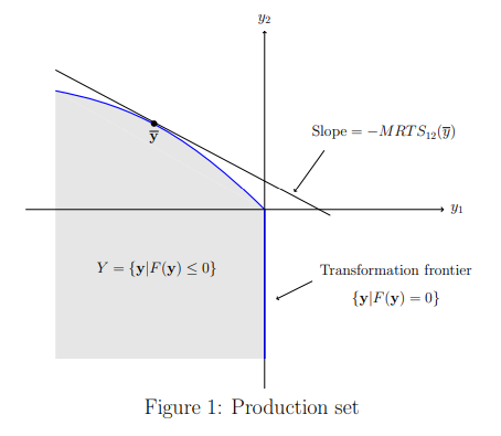
transformation function: .
production set: .
input requirement set: .
production function: .
Isoquant inputs: .
production set when is given: .

Elasticity of Substitution

Definition (Elasticity of Substitution).

Elasticity of Substitution between inputs and at the point is the larger is, the easier substitution between inputs and .

Example (CES production function).

For CES production function Since we have , this implies that thus, elasticity of substitution is, which is a constant.

Example (transformation of CES function).

For CES production function some well-known production functions belong to the CES class:

if , then (linear)
if , then (Cobb-Douglas)
if , then (Leontief)

Proof.Let the CES function be

If , it is trivial since
Let .
- by taking log on both sides,
- by the L'hospital's law,
- thus we have
- by taking exponential on both sides to get the original function, thus it is a Cobb-Douglas function.
Let .
- Similar to the prior proof, first take log on both sides:
- Let . then by the L'hospital's law,
- where the last equation holds since
- therefore, we have which is a Leontief function.

this completes the proof. □

Properties of Production Sets

Let be the set of all inputs and outputs. We Assume that the production sets satisfies the following properties:

is nonempty: at least contains (produce nothing)
is closed: boundary is included
No free lunch: no inputs, no outputs or, .
Possibility of inaction: sunk cost is ignored
Free disposal: no cost to through away the remaining inputs or outputs
is convex: balanced combination of production is preferred

Definition (Return to Scale).

A production function has the property of:

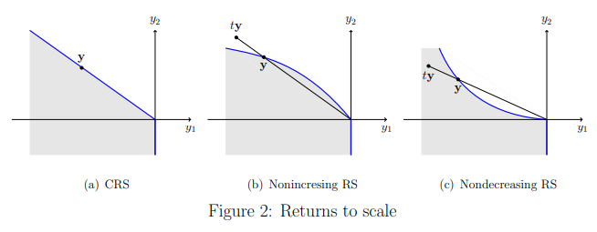
constant returns to scale (crs) if for .
increasing returns to scale (irs) if for .
decreasing returns to scale (drs) if for .
non-increasing returns to scale (nirs) if for , or
non-decreasing returns to scale (ndrs) if for , or

Proposition (convexity implies nirs).

If is convex and inaction is allowed, then is nonincreasing return to scale(nirs).

Proof.Since is possible of inaction, we have . then by convexity of , we have i.e. is nirs. □

Profit Maximization

Assume:

competitive market: firms are the price takers
is nonempty, closed, and free disposal.

Profit Maximization Problem (PMP)

Proposition (PMP).

For , the firm's Profit Maximization Problem (PMP) is If one output and inputs, we have where is output price and is input price vector.

Proof.From PMP, Then the Lagrangian is, F.O.C. i.e. Thus MRTS is,

Now, let there be one output and inputs. than from PMP, then the Lagrangian is F.O.C. thus This implies that

this completes the proof. □

Profit Function

Definition (profit function and supply correspondence).

Let is a price vector. then is a profit function, where is a supply correspondence, the set of profit-maximizing production plans.
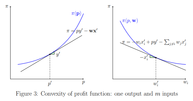
In the case of one output and inputs, the supply correspondence can be represented as, where is output supply function and is factor demand functions.

Theorem (Properties of Profit function).

If is closed and satisfies the free disposal, then

If for all output and for all input . then .
is homogeneous of degree one, while is HOD0.
is convex in .

Proof.

Let for all output, i.e. . and for all inputs for which . thus we have thus we have
WTS#1 is HOD0: WTS#2 is HOD1:
by Def (convex function)Def (convex function), WTS by letting , we have where inequality holds due to the definition of .

this completes the proof. □

Pasted image 20240405213014.png

Theorem (Hotelling's lemma).

For all , i.e.

Proof.Assume is differentiable, and let and define a function and note that Thus, the first-order-conditions for a minimum at requires therefore we have which is equivalent to this completes the proof. □

Remark (substitution matrix).

If is differentiable, then the supply substitution matrix is symmetric and positive semidefinite. which implies the law of supply,

Proof.WTS is symmetric and positive semidefinite.

By the ^b7e327 Theorem 10 (Hotelling's lemma), we have which means that is symmetric.
Since is convex, we have i.e. is positive semidefinite.

Furthermore, let are the price vectors, where and . then we have which add up to which means for for , we have this completes the proof. □

Cost Minimization

Cost Minimization Problem (CMP)

Proposition (CMP).

for and , Cost Minimization Problem(CMP) is defined as and the solution exists if is closed, and a set of solutions is convex if is convex.

Proof.From CMP, the Lagrangian function is F.O.C. thus we have .
Therefore, by letting be the optimal CMP, we have this implies that and this completes the proof. □

Properties of Cost Function

Definition (cost function).

Let is input price vector and is output level with . then the cost-minimizing input vector is which is called conditional factor demand function.
and the cost function of the firm is furthermore, the marginal cost is which indicates the marginal cost required for the one additional output.

Theorem (properties of cost function).

If is continuous and strictly increasing, then is

homogeneous of degree 1 in .
strictly increasing in and nondecreasing in .
concave in .
continuous in and .

Proof.The proof is identical to Basic Consumer Theory > ^6bcfb6 Basic Consumer Theory > Proposition 29 (Properties of the Expenditure Function).

WTS :
WTS , and , .
1. First we show the strictly increasing in .
  - RTA: ASM is not strictly increasing in : where and .
  - let for some .
  - since is continuous, we have
  - this contradicts to the assumption that , since is not a CMP solution for given .
2. Next we show the nondecreasing in .
  - ASM: .
  - then we have
for a fixed , let and . WTS
- as is the CMP for any , we have
- therefore, we have
- thus is concave in .
This directly follows from Berge's Maximum TheoremBerge's Maximum Theorem.
- note that where is the solution of CMP.
- if is continuous, than is also continuous.

this completes the proof. □

Theorem (Shephard's lemma(cost function)).

For all , i.e.

Proof.Assume is differentiable in , and let and define a function and note that Thus, the first-order-conditions for a minimum at requires therefore we have which is equivalent to this completes the proof. □

Solving PMP and CMP

Remark (alternative expression of the PMP).

Given the cost function , the alternative expression of PMP is where the first-order condition is

Example (Profit and Cost Function for Cobb-Douglas function).

Let the Cobb-Douglas production function be

Proof.We first derive the cost function from CMP, and second, we derive the factor demand function and the profit function from PMP.

From CMP: Lagrangian: F.O.C. thus we have which implies .

From the above equality, we have therefore, the conditional factor demand function is furthermore, the cost function is where denotes per unit cost of production.

From PMP: since and , PMP is F.O.C. which is a sufficient condition when .

Case 1) (Decreasing Returns to Scale; DRS)
the supply function is as , we have and finally, the profit function is

Case 2) (Constant Returns to Scale; CRS)
From F.O.C., the right hand side becomes the unit cost of production, which is independent to .

if : is optimal
if : no solution exists (unbounded profits)
if : any is solution for PMP where .

Case 3) (Increasing Returns to Scale; IRS)
From F.O.C., such satisfying the inequality is not the solution for PMP, since is strictly concave in . therefore any satisfying F.O.C. is local minimum profits.

this completes the proof. □

Short-run and Long-run CMP

Definition (short-run and long-run CMP).

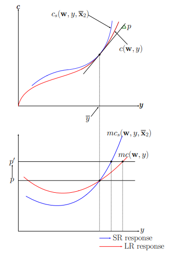
Assume that some inputs are fixed at . Then the firm's short-run cost minimization problem is where

: short-run conditional factor demand function.
: short-run cost function
: short-run variable cost
: short-run fixed cost.

Proposition (relation between short-run and long-run).

Let are given, and be the long-run cost minimizing level. then we have the following relations: where

long-run (average) cost curve is the lower envelope of the short-run (average) cost curves.
the response of output to its price change is greater in the long-run than in the short-run.

Proof.for given some , let . and define then is maximized at . since for any , we have , thus as is long-run CMP.

therefore, the first and second order conditions imply and, which completes the proof. □

Pasted image 20240409220702.png

Duality

Theorem (CMP given output equals to PMP given cost).

Let be a cost function from and define and let be a cost function from . then we have

This theorem implies

cost function summarizes all of the economically relevant aspects of the technology.
the technology recovered from the cost function is essentially the same as the true technology.

Proof.First, by definition of and since is a cost function from , we have Next, if , then by the definition we have and therefore, we have . which implies .
thus we concludes that this completes the proof. □

Theorem (duality of PMP and CMP).

If any function satisfies all the properties of cost function is ^74ef56 Theorem 14 (properties of cost function), then it is indeed a cost function for the technology defined by
If any function satisfies all the properties of conditional factor demand function, then it is actually the conditional factor demand function.

Example (Cobb-Douglas function).

Consider

Proof.First, by applying ^7d55d9 Theorem 15 (Shephard's lemma(cost function)), thus we have therefore, we obtain which is C-D technology. □